Tutorial

This tutorial introduces the reader to particle-based simulations of nanomotors. The main simulation method consists of a coupled scheme of Multiparticle Collision Dynamics (MPCD), for the fluid, and Molecular Dynamics (MD), for the motor. Chemical activity is introduced in the fluid via a surface-induced catalytic effect and bulk kinetics.

To start working with RMPCMD, visit the Install section first.

Introduction

Nano- to micro-meter scale devices that propel themselves in solution are built and studied since about a decade. They represent a promise of future applications at scales where usual control strategies reach their limits and, ideally, autonomous action replaces manual control.

It is possible to compute, via phoretic theory, the stationary regime of operation of nanomotors in simple geometries. Still, testing geometrical effects or including fluctuating behaviour is best done using numerical simulations. A successful modeling strategy was started by Rückner and Kapral in 2007 [RK07]. It builds on a particle-based fluid, explicitly the Multiparticle Collision Dynamics (MPCD) algorithm. The flexibility of particle-based simulations allowed for numerous extensions of their work to Janus particles, polymer nanomotors, various chemical kinetics, thermally active motors, among others.

The principle of the hybrid scheme is very close to full Molecular Dynamics (MD), with the major difference that solvent-solvent interactions are not explicitly computed and are replaced by cell-wise collisions at fixed time intervals. This saves computational time and renders otherwise untractable problems feasible.

In Ref. [RK07], the authors introduce a computational model for a dimer nanomotor that is convenient thanks to its simple geometry. There are two spheres making up the dimer, linked by a rigid bond, one of which being chemically active and the other not. Solvent particles in contact with the chemically active sphere are converted from product to fuel. The active sphere thus acts as a sink for reagent particles (the “fuel”) and a source for product particles.

Preliminary remarks

This tutorial does not intend to cover all possible manners to conduct nanomotor simulations. Rather, it aims at presenting one strategy for modeling chemically powered nanomotors, that is the combination of a chemically active MPCD fluid coupled to possibly catalytic colloidal beads.

While this tutorial relies on the RMPCDMD software, it is worth mentioning that Peter Colberg has also made his software for dimer nanomotor simulations available openly [Col15]. nano-dimer is based on OpenCL and can benefit from GPU acceleration.

Literature

The MPCD algorithm was introduced in [MK99] and [MK00]. General reviews on the MPCD simulation method are available in the literature.

• Raymond Kapral, Multiparticle collision dynamics: simulation of complex systems on mesoscales, Adv. Chem. Phys. 140, 89 (2008). [Kap08]

• G. Gompper, T. Ihle, D. M. Kroll and R. G. Winkler, Multi-Particle Collision Dynamics: A Particle-Based Mesoscale Simulation Approach to the Hydrodynamics of Complex Fluids, Adv. Polymer Sci. 221, 1 (2008). [GIKW08]

An overview of chemically powered synthetic nanomotors has been published by Kapral [Kap13].

There is no literature on the practical conduct of nanomotor simulations, however.

The MPCD fluid and Molecular Dynamics

A MPCD fluid consists of point particles with a mass (set to unity here for convenience), a position \(x\) and a velocity \(v\). The particles evolve in two step: (i) indepedent streaming of the particles for a duration \(\tau\) and (ii) cell-wise collision of the particles’ velocities.

For particle \(i\) this results in the following equations:

(1)\[x_i' = x_i + v_i \tau\]

and

(2)\[v_i' = v_\xi + \omega_\xi ( v_i - v_\xi )\]

where the prime denotes the quantities after the corresponding step, \(\xi\) is a cell, \(\omega_\xi\) is a rotation operator and \(v_\xi\) is the center-of-mass velocity in the cell. The cell consists in a regular lattice of cubic cells in space. Equations (1) and (2) conserve mass, energy and linear momentum.

The viscosity for a MPCD fluid can be computed from its microscopic properties:

\[\eta = \frac{k_BT\tau\rho}{2m} \left( \frac{ 5\gamma - (\gamma-1+e^{-\gamma})(2-\cos\alpha-\cos 2\alpha) }{(\gamma - 1 + e^{-\gamma})(2-\cos\alpha-\cos 2\alpha)} \right) + \frac{m}{18 a \tau} (\gamma -1 + e^{-\gamma})(1-\cos\alpha)\]

One can embed a body in a MPCD fluid by using a explicit potential energy. Then, the streaming step is replaced by the velocity-Verlet integration scheme. Collision involve only fluid particles and not the colloid.

The dimer nanomotor

Physical setup

In this section, we review the propulsion of the dimer nanomotor presented by Rückner and Kapral. The geometry of the motor and the chemical kinetics are presented in Fig. 1.

The solvent consists of particles of types A and B, initially all particles are set to A (the fuel). Fuel particles that enter the interaction range of the catalytic sphere are flagged for reaction but the actual change of A to B only occurs when the solvent particle is outside of any interaction range. Else, the change would generate a discontinuous jump the in the potential energy and disrupt the trajectory. This chemical activity generates an excess of product particles “B” around the catalytic sphere and a gradient of solvent concentration is established.

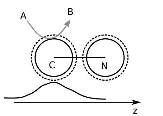
Fig. 1 Geometry and chemistry for the dimer nanomotor. The graph sketched below represents the local excess of “B” particles that is asymmetric for the “N” sphere. Many more “A” and “B” particles not shown.

In this type of simulation, the total energy is conserved but the system is maintained in nonequilibrium by refueling, that is by changing B particles to species A when they are far enough from the colloid.

The solvent and colloids interact via a purely repulsive Lennard-Jones potential of the form

\[V(r) = 4 \epsilon \left( \left(\frac{\sigma}{r}\right)^{12} - \left(\frac{\sigma}{r}\right)^{6} - 1 \right)\]

where \(\epsilon\) and \(\sigma\) can be different depending on the combination of solvent and colloid species.

Simulation setup

Within RMPCDMD, the simulation program for the dimer is called single_dimer_pbc. This program requires a configuration file that contains the physical parameters, an example of which is given in the listing below.

# physical parameters
T = .16666666
L = 32 32 32
rho = 9
tau = 1.0
probability = 1.0
bulk_rmpcd = F
bulk_rate = 0.001

# simulation parameters
N_MD = 200
N_loop = 50
equilibration_loops = 50
colloid_sampling = 50

# interaction parameters
sigma_N = 4.0
sigma_C = 2.0

d = 6.8
epsilon_N = 1.0 0.1
epsilon_C = 1.0 1.0

epsilon_N_N = 1.0
epsilon_N_C = 1.0
epsilon_C_C = 1.0

The configuration allows one to set the size of both spheres in the dimer as well as the interaction parameters. The setting epsilon_N contain the prefactor to the Lennard-Jones potential for the “N” sphere and all solvent species on a single line. In this example, all the interaction parameters are set to 1 except for the interaction between the “N” sphere and “B” solvent particles, as was done in [RK07].

Running the simulations

Note

Make sure that you have built the code properly (see Install) and that the command-line tool rmpcdmd is available at your command-line prompt. You will also need a working scientific Python environment (see Python).

An example simulation setup is provided in the directory experiments of RMPCDMD. There, the sub-directory 01-single-dimer contains a parameter file.

Review the parameters in the file dimer.parameters then execute the code

make dimer.h5

The actual commands that are executed will be shown in the terminal.

Analyzing the data

The output of the simulation is stored in the file dimer.h5, that follows the H5MD convention for storing molecular data [dBCH14]. H5MD files are regular HDF5 files and can be inspected using the programs distributed by the HDF Group. Issue the following command and observe the output:

h5ls dimer.h5

HDF5 files have an internal directory-like structure. In dimer.h5 you should find

fields                   Group
h5md                     Group
observables              Group
parameters               Group
particles                Group
timers                   Group

The elements are called “groups” in HDF5 terminology. Here, there is data about the particles (positions, velocities, etc), observables (e.g. temperature) and fields (here, the histogram of “B” particles). The h5md group contains metadata (simulation creator, H5MD version, etc.), the timers group contains timing data that is collected during the simulation and parameters contains all the parameters with which the simulation was run.

The command

h5ls -r dimer.h5

will visit all groups recursively. The output is then rather large. Let us focus first on the velocity of the dimer, it is located at /particles/dimer/velocity, where it is stored in value and the time step information of the dataset is stored in step and time. In the present case, the velocity is sampled at regular time interval of 100 timesteps or equivalently 1 in units of \(\tau\).

All the data analysis in this tutorial is done using the Python language and a set of libraries: NumPy for storing and computing with array data, h5py for reading HDF5 files, matplotlib for plotting and SciPy for some numerical routines. For installation, see appendix [install-py]. Some generic programs are provided with as an introduction to reading the files, such as h5md_plot.py. Its usage is

rmpcdmd plot dimer.h5 --obs temperature

(the obs option is preceded by two dashes) to display the temperature in the course of time. This program can also display the trajectory of the dimer

rmpcdmd plot dimer.h5 --traj dimer/position

More specific information on the dimer nanomotor can be obtained via Python programs located in the experiments/01-single-dimer directory.

The directed velocity, that is the velocity in the direction of the motor’s propulsion axis, can be obtained via

python plot_velocity.py dimer.h5 --directed

A further option --histogram show an histogram instead of the time-dependent value.

Finally, an important quantity to assess both for theory and experiments is the effective diffusion that results from both thermal fluctuations and the combination of self-propelled motion and random reorientation.

python plot_msd.py dimer.h5

This latter program can take several simulation files as input to obtain better statistics. It is also important to use a much simulation time (N_loop) than the default one to produce meaningful results.

The Janus nanomotor

A Janus motor comprises two hemispheres with one chemically active surface and one inactive surface as shown in Fig. 2 (a). Because chemical reactions happen asymmetrically on the Janus motor surface, a concentration gradient of product particles is generated giving rise to self-propulsion. In 2013, de Buyl and Kapral introduced a composite model for Janus motor [dBK13], see Fig. 2 (b). The active (blue, C) and inactive (red, N) parts are composed of spheres linked by rigid bonds. These spheres have the same radius, and interact with the surrounding solvent particles through repulsive Lennard-Jones potentials \(V_{\alpha C}\) and \(V_{\alpha N}\), where \(\alpha = A, B\) is the type of solvent species.

An example simulation setup for self-proplusive Janus motor is provided in the directory experiments/03-single-janus. The parameter file is show below:

# physical parameters
T = .333333333
L = 32 32 32
rho = 9
tau = 1.0
probability = 1

# simulation parameters
N_MD = 100
N_loop = 512
colloid_sampling = 50
equilibration_loops = 20
data_filename = janus_structure.h5
link_treshold = 2.5
do_read_links = F
polar_r_max = 10
bulk_rate = 0.1

# interaction parameters
sigma_colloid = 2
epsilon_colloid = 2
do_lennard_jones = T
do_elastic = F
do_rattle = T
rattle_pos_tolerance = 1d-8
rattle_vel_tolerance = 1d-8

sigma = 3
epsilon_N = 1.0 5.0
epsilon_C = 1.0 1.0

To run the simulation, use make simulation, and check the propulsion speed \(V_z\) with

python plot_velocity.py janus.h5 --directed

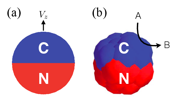
Fig. 2 (a) The sketch of a Janus particle with active (C) and inactive (N) hemispherical surface moving along particle axis with velocity \(V_z\). (b) The composite model for Janus particle. Chemical reactions, \(A \to B\), take place at the active surface.

Controls of motor speed

For Janus particles, one can obtain from phoretic theory that the propulsion speed is determined by factors such as the system temperature, fluid properties (viscosity and density) but also the chemical kinetics and the specific solvent-colloid interactions [Kap13].

In this section, we explore the effects of the interaction parameters and of the reaction rate \(k_2\) on the direction and strength of the propulsion. By modifying only the lines below in the parameter file for the janus simulation, it is possible to observe a reversal of propulsion and the effect of the reaction rate \(k_2\).

Example 1, forward moving Janus motor.

epsilon_N = 1.0 0.5
epsilon_C = 1.0 0.5
bulk_rate = 0.001

Example 2, backward moving Janus motor.

epsilon_N = 0.5 1.0
epsilon_C = 0.5 1.0
bulk_rate = 0.001

Example 3, changing the bulk reaction rate.

epsilon_N = 1.0 0.5
epsilon_C = 1.0 0.5
bulk_rate = 0.0001