Correlation functions

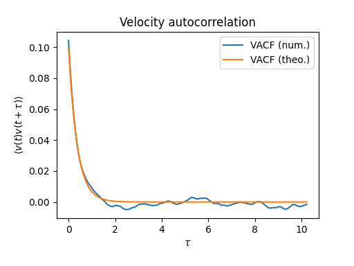
Generate the velocity for a Ornstein-Uhlenbeck process and compute its autocorrelation function.

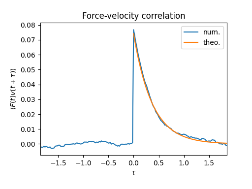
We also display the force velocity correlation as an example of using the routine correlation.

• 
• 

import numpy as np
import tidynamics
import matplotlib.pyplot as plt

plt.rcParams['figure.figsize'] = 5.12, 3.84
plt.rcParams['figure.subplot.bottom'] = 0.18
plt.rcParams['figure.subplot.left'] = 0.16

# Generate data for a Ornstein-Uhlenbeck process

gamma = 2.7
T = 0.1
dt = 0.02
v_factor = np.sqrt(2*T*gamma*dt)

N = 32768
v = 0
for i in range(100):
    noise_force = v_factor*np.random.normal()
    v = v - gamma*v*dt + noise_force

v_data = []
noise_data = []

for i in range(N):
    noise_force = v_factor*np.random.normal()
    v = v - gamma*v*dt + noise_force
    v_data.append(v)
    noise_data.append(noise_force)
v_data = np.array(v_data)
noise_data = np.array(noise_data)/np.sqrt(dt)

# Compute the autocorrelation function and plot the result

acf = tidynamics.acf(v_data)[:N//64]

time = np.arange(N//64)*dt

plt.plot(time, acf, label='VACF (num.)')

plt.plot(time, T*np.exp(-gamma*time), label='VACF (theo.)')

plt.legend()
plt.title('Velocity autocorrelation')
plt.xlabel(r'$\tau$')
plt.ylabel(r'$\langle v(t) v(t+\tau) \rangle$')

# Compute the force velocity correlation and plot the result

plt.figure()

time = np.arange(N)*dt
twotimes = np.concatenate((-time[1:][::-1], time))

plt.plot(twotimes, tidynamics.correlation(noise_data, v_data),
         label='num.')
plt.plot(time, 2*T/gamma*np.exp(-gamma*time), label='theo.')

plt.xlim(-5/gamma, 5/gamma)

plt.ylim(-2*T/gamma/10, 1.1*2*T/gamma)

plt.legend()
plt.title('Force-velocity correlation')
plt.xlabel(r'$\tau$')
plt.ylabel(r'$\langle F(t) v(t+\tau) \rangle$')

plt.show()