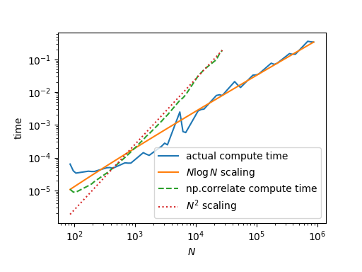
Scaling behaviour

Compute the autocorrelation for varying time series lengths.

The figure displays the timing and a \(N log N\) scaling law, demonstrating the claimed complexity.

import numpy as np
import tidynamics
import matplotlib.pyplot as plt
import time

plt.rcParams['figure.figsize'] = 5.12, 3.84
plt.rcParams['figure.subplot.bottom'] = 0.18
plt.rcParams['figure.subplot.left'] = 0.16


all_N = []
N = 64
for i in range(14):
    all_N.append(N + int(N/3))
    all_N.append(N + int(N/2))
    all_N.append(N + int(2*N/3))
    N = 2*N
all_N = np.array(all_N)

max_direct_N = 32768
all_time = []
direct_time = []
n_runs = 5

for N in all_N:
    t = 0
    direct_t = 0
    for i in range(n_runs):
        data = np.random.random(size=N)
        t0 = time.time()
        acf = tidynamics.acf(data)
        t += time.time() - t0
        if N <= max_direct_N:
            t0 = time.time()
            acf = np.correlate(data, data, mode='full')
            direct_t += time.time() - t0

    all_time.append(t/n_runs)
    if N <= max_direct_N:
        direct_time.append(direct_t/n_runs)

plt.plot(all_N, all_time, label='actual compute time')
plt.plot(all_N,
         all_time[-1] * all_N*np.log(all_N) / (all_N[-1]*np.log(all_N[-1])),
         label=r'$N\log N$ scaling')
plt.plot(all_N[:len(direct_time)], direct_time,
         label='np.correlate compute time', ls='--')

data_len = len(direct_time)
plt.plot(all_N[:data_len],
         all_N[:data_len]**2 * direct_time[data_len-1] / all_N[data_len-1]**2,
         label=r'$N^2$ scaling', ls=':')

plt.xlabel(r'$N$')
plt.ylabel('time')

plt.loglog()
plt.legend()

plt.show()