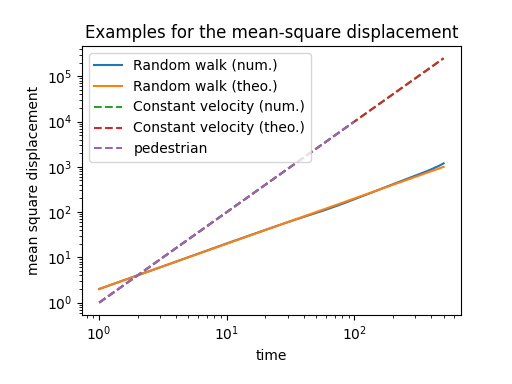
Mean-square displacements (MSD)

Generate a number of random walks and compute their MSD.

Compute also the MSD for a constant velocity motion.

For a random walk, the MSD is linear: \(MSD(\tau) \approx 2 D \tau\)

For a constant velocity motion, the MSD is quadratic: \(MSD(\tau) = v \tau^2\)

We show in the figures the numerical result computed by tidynamics.msd (‘num.’) and the theoretical value (‘theo.’).

For the constant velocity case, we also display a “pedestrian approach” where the loop for averaging the MSD is performed explicitly.

import numpy as np
import tidynamics
import matplotlib.pyplot as plt

plt.rcParams['figure.figsize'] = 5.12, 3.84
plt.rcParams['figure.subplot.bottom'] = 0.18
plt.rcParams['figure.subplot.left'] = 0.16

# Generate 32 random walks and compute their mean-square
# displacements

N = 1000
mean = np.zeros(N)
count = 0
for i in range(32):
    # Generate steps of value +/- 1
    steps = -1 + 2*np.random.randint(0, 2, size=(N, 2))
    # Compute random walk position
    data = np.cumsum(steps, axis=0)
    mean += tidynamics.msd(data)
    count += 1

mean /= count
mean = mean[1:N//2]

time = np.arange(N)[1:N//2]

plt.plot(time, mean, label='Random walk (num.)')

plt.plot(time, 2*time, label='Random walk (theo.)')

time = np.arange(N//2)

# Display the mean-square displacement for a trajectory with
# constant velocity. Here the trajectory is taken equal to the
# numerical value of the time.

plt.plot(time[1:], tidynamics.msd(time)[1:],
         label='Constant velocity (num.)', ls='--')
plt.plot(time[1:], time[1:]**2,
         label='Constant velocity (theo.)', ls='--')

# Compute the the mean-square displacement by explicitly
# computing the displacements along shorter samples of the
# trajectory.

sum_size = N//10
pedestrian_msd = np.zeros(N//10)
for i in range(10):
    for j in range(N//10):
        pedestrian_msd[j] += (time[10*i]-time[10*i+j])**2
pedestrian_msd /= 10
plt.plot(time[1:N//10], pedestrian_msd[1:], ls='--',
         label="pedestrian")

plt.loglog()
plt.legend()
plt.xlabel('time')
plt.ylabel('mean square displacement')
plt.title('Examples for the mean-square displacement')
plt.show()